Happy EconEdMonth! Celebrate economics all month long by visiting EconEdMonth.org

Nearpod version available

Grade 9-12
,
Lesson

Using Slope to Compute Opportunity Cost

Time: 60 mins,
Updated: October 17 2023,

Objective

Students will be able to:

  • Define slope and opportunity cost.
  • Compute the slope between two points.
  • Use slope to interpret opportunity cost.

In this personal finance lesson, students will investigate opportunity cost by using slope.

Resources

Procedure

The concept of opportunity cost is a foundation of economic study, and while advanced mathematics is generally used to compute it from a production possibilities frontier, the computation of slope (“rise over run”) can be used to approximate the opportunity cost by using production possibilities curves. Students will be using their math skills to compute the slopes of various production possibilities frontiers in order to determine the opportunity cost of producing different combinations of two goods. Ultimately, students will move from computing slope on a linear production possibilities frontier to one that is concave to the origin where the slope changes. This lesson is best taught in a high school Introductory Algebra course. The teacher should note that this lesson does not cover all aspects of slope. For example, all of the slopes examined in this lesson, due to the nature of the production possibilities frontier, are negative. Further, the slopes are located exclusively in the first quadrant of the coordinate plane. However, the lesson is designed to teach students a practical application of slope.

  1. Begin class by asking students how they choose to allocate their time after school.
    [Answers will vary, but will likely include spending time with friends, doing homework, playing games, etc. Write all responses on the board.]
  2. Explain that students have a constraint—the amount of time available after school and before they must go to bed. If they spend that time doing one thing, they can’t spend it doing something else. Point out that if you spend your time after school grading papers, you can’t spend your time at the gym—going to the gym is your opportunity cost. Ask a student how s/he would spend an hour after school and what the opportunity cost of that hour would be.
    [Answers will vary, but students should recognize that as they spend an hour playing games, they give up the next highest-valued use of that hour.]
  3. Display Slide 1 for the students. Explain that economists use a model called a production possibilities frontier. Define production possibilities frontier as a graph showing the combination of two goods, which can be produced given current resources and technology.
  4. Explain that the production possibilities frontier is a model with the following assumptions: an economy is producing only two goods, the amount of resources available (labor, capital, and natural resources) remain constant, and technology remains constant. Using Slide 1 as a guide, walk students through the key components of a production possibilities frontier.
    • The two endpoints on the axes indicate the points where the producer is making all of one good and none of the other. For example, this producer can make 60 chips and zero fish or 30 fish and zero chips.
    • Any point along the curve is a combination of fish and chips which this producer can make given current technology and resources.
  5. Distribute a copy of Activity 1 to each student. Instruct students to create their own production possibilities frontier. Ask the following questions to check for understanding:
    1. What is happening at each of the endpoints of the line?
      [Utopia is producing all of one good and none of the other good.]
    2. What is happening at any point along the line?
      [Utopia is producing a mixture of cars and trucks.]
    3. What is one possible combination of cars and trucks that Utopia can produce in each graph (1 through 4)?
      [There are numerous correct responses, and answers will vary for each graph. Check student responses with the graph for accuracy. Students should be choosing points that lie along or below the production possibilities frontier.]
    4. What assumptions are we making about technology and resources in Utopia?
      [They remain constant.]
  6. Point out that points outside the frontier cannot be reached with current technology, while points inside the frontier can be produced but some resources are not being used—that is there is unemployment (people aren’t working, factories are empty) or inefficiency (points along the curve represent technological efficiency). If technology improves, production can occur outside the production possibility curve.
  7. Show Slides 2 through 6 and explain the definition of slope with the formula vertical change/horizontal change, often referred to as “rise over run.” Explain to students that slope measures the steepness, or rate of change, of the line.
    • Use Slide 3 to demonstrate the mathematical computation of slope. The “rise over run” expression is a simple and direct way to teach the concept.
    • Use Slide 4 to explain that slope measures the rate of change from one point to the next. This concept will be important throughout the lesson, as students use the production possibilities frontier model.
    • Use Slides 5 through 7 to guide students through the mathematics.
  8. Show Slide 8 and have students practice slope problems independently. Circulate around the room to check student responses to these questions.
    [Question 1: 7/6; Question 2: -3/4; Question 3: -4/5; Question 4: 6/5; Question 5: 0]
  9. Explain that slope is related to an important concept in economics called opportunity cost. Explain that opportunity cost is the value of the next best alternative given up when a decision is made. Using the production possibilities frontier from Slide 1, show that as more chips are produced, a certain number of fish must be given up. Conversely, as more fish are produced, some chips are given up. Reinforce that the exact amount of one good sacrificed to gain the other is the opportunity cost, and is represented by the slope of the line.
  10. Explain that students will be using slope to identify opportunity cost.
  11. Distribute a copy of Activity 2 to each student. Have students complete the activity. Review student answers.
    1. What is the slope of the line?
      [Graph 1: -1; Graph 2: -¾; Graph 3: -2]
    2. In Graph 1, what is the opportunity cost of producing 20 trains?
      [20 airplanes]
    3. In Graph 1, what do you notice about the relationship between the number of trains given up and the number of airplanes gained?
      [Students should note that for every train given up, one airplane is gained and vice versa.]
    4. In Graph 1, what is the relationship between slope and opportunity cost?
      [Slope is a mathematical way of expressing opportunity cost; the slope of the line over a given segment of the production possibilities frontier corresponds to the opportunity cost between those two goods. Be sure students recognize that the slope of Graph 1 is -1/1, which corresponds to the one-to-one ratio identified in question c above.]
  12. Review with students the answers to Graphs 2 and 3, asking the same questions (a-d) with each graph.
    [Reinforce that slope corresponds to the opportunity cost. For instance, in Graph 3 the slope is -2. Students should respond that for every one football produced, two basketballs must be sacrificed. Be sure to point out that opportunity cost works the other way as well: for every basketball produced, ½ of a football is given up. This concept of “½ of a basketball” might be confusing to students; remind them that opportunity cost and production possibilities frontiers are theoretical models.]
  13. Distribute a copy of Activity 3 to ¼ of the students, Activity 4 to ¼ of the students, Activity 5 to ¼ of the students, and Activity 6 to ¼ of the students. Give students time to compute the slope of their respective section of the production possibilities frontier.
  14. Project Slide 9 for the students. Ask a representative of each group to come to the front of the room. Ask the following questions to check for understanding:
    1. How is the shape of this production possibilities frontier different than the previous ones?
      [This PPF, instead of being linear, is concave to the origin, i.e., “bowed out.”]
    2. What is the slope of each section of the graph?
      [Section A to B: -3/4; Section B to C: -1; Section C to D: -4/3; Section D to E: -5]
    3. What do you notice about the various slopes of each section?
      [Students should notice that the slopes between the points are changing.]
    4. What does this indicate about opportunity cost?
      [Students should recognize that opportunity cost is changing as production moves along the production possibilities frontier.]
  15. Explain to students that real production possibilities frontiers are rarely straight lines, and tend to resemble the bowed out ones they have just completed with changing opportunity cost. Ask students to speculate why the opportunity cost between producing radios and producing TVs could change.
    [Answers will vary, but guide students to the idea that resources are not perfect substitutes for each other.]
  16. Explain that as we make more televisions the tools we are using to make radios are not quite as efficient as they were, increasing our opportunity cost; essentially, we have to give up more of radios to gain fewer televisions.
  17. Conclude the lesson by asking the following questions:

a, Ask students to define slope and opportunity cost.
                    [Slope is the rate of change or steepness of the line; opportunity cost is the highest valued alternative that must be given up to gain something else.]

b. Refer students to Slide 1 and review the computation of slope, specifying the “rise over run” calculation.

c. Ask students to state the relationship between slope and opportunity cost.
                          [Students should state that slope is a mathematical expression of opportunity cost and shows the quantity of goods which must be given up to gain more of the other good.]

Assessment

Multiple Choice

  1. Which of these best describes the concept of slope?
    1. [A mathematical formulation of the steepness of a line.]
    2. An expression of the curvature of a line.
    3. A function of two variables used to solve inequalities.
    4. An algebraic notation of absolute value.
  2. Barney and his friends enjoy doing two things: painting pictures and writing poetry. However, they must allocate their time. If they are doing one activity, they cannot be doing the other. Barney and his friends have the following points on their production possibilities frontier (the first number represents the number of pictures painted, the second the number of poems written): (5, 15) and (3, 29). Which of these expresses Barney’s opportunity cost?
    1. Give up 1 painting to write 5 poems.
    2. [Give up 1 painting to write 7 poems.]
    3. Give up 1 poem to paint 2 pictures.
    4. Give up 1 poem to paint 4 pictures.
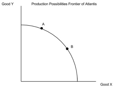
  3. At a given Point A on the production possibilities frontier, Atlantis has a slope of -1/3 between Good X and Good Y. At Point B on the production possibilities frontier, Atlantis has a slope of -1. Assuming we are moving production from Point A to Point B, which of the following best describes the opportunity cost of choosing more of Good X?

  1. [The opportunity cost is increasing.]
  2. The opportunity cost is decreasing.
  3. The opportunity cost is constant.
  4. The opportunity cost is positive.

Constructed Response

  1. Imagine you are the Chief Production Officer at a factory which can make two toys: plastic dolls and teddy bears. You have been given the task by the owner of the factory to model the use of inputs in producing both products.
    1. Assume that the same resources can be used to make teddy bears or plastic dolls. If you put all available resources into making plastic dolls, you can manufacture 160. If you focus only on making teddy bears, you can manufacture 20. Draw a linear production possibilities frontier and calculate the slope.
    2. Using your data from part a, give any two combinations of plastic dolls and teddy bears which would also be feasible to produce.
      [Answers will vary, but must fall between the outer bounds of production given in Part A and still maintain the same slope generated in Part A.]
    3. Explain why the production possibilities frontier between plastic dolls and teddy bears is not likely to be linear.
      [Resources used to make teddy bears, such as soft stuffing and thread, are not likely to be efficient in making hard plastic dolls. Thus, if the factory converts from making one good to making the other, they will have to give up more and more to gain fewer and fewer.]
Subjects:
Economics,Math